
Status: draft. Verified steps and screenshots to come.
In this lesson you will draw formaldehyde's electron density and its highest occupied orbital as surfaces in ParaView, choosing the surface value yourself. Time: 15 minutes · Branch: Densities and volumes · Program: ParaView · Also in: GaussView, ChimeraX, PyMOL
| Before this | Data | You'll need |
|---|---|---|
| Start ParaView on OnDemand | Formaldehyde's density.cube and homo.cube in ~/scratch/cubes: get the cube files |
A running ParaView session |
Note
Cluster details. Highlighted values are placeholders. AMA27's queue names, module versions, paths and addresses go in when the cluster is deployed.
Why this matters
Quantum-chemistry programs compute numbers on a 3-D grid: the electron density, orbitals, the electrostatic potential. A cube file stores that grid. ParaView reads it as it reads any other volume, so the filters and color maps from the simulation lessons apply unchanged. The same pipeline, saved as a script, redraws the picture for the next molecule.
Key idea
A surface shows where a value is reached. An isosurface is the surface where the grid equals one chosen number, its isovalue, so the number decides the shape. For the density, 0.0004 e/bohr³ gives a surface about the size of the molecule and 0.05 hugs the atoms and bonds. An orbital takes positive and negative values, so it needs two surfaces, 0.02 and -0.02, drawn in two colors. Here you draw the HOMO, the highest occupied orbital. The topic page explains the idea in full.
Steps
Step 1: Open the density
Choose File ▸ Open…, open ~/scratch/cubes/density.cube, and click Apply.
You should see: under density.cube in the Pipeline Browser, two outputs: Molecule (the atoms) and Gridded Data (the numbers). ParaView 6 splits the file this way; in ParaView 5 the reader gives the grid alone.
Screenshot: the Pipeline Browser with the Molecule and Gridded Data outputs
Screenshot to come: The Pipeline Browser showing density.cube with its two outputs, Molecule and Gridded Data
Step 2: Draw the density surface
Select Gridded Data. Choose Filters ▸ Alphabetical ▸ Contour, set Isosurfaces to 0.05, and click Apply.
You should see: a surface around the atoms. Change the value to 0.0004 and click Apply: the surface swells to about the molecule's full size. Set it back to 0.05.
Screenshot: Contour's properties, with Isosurfaces marked
Screenshot to come: The Properties panel for Contour1, with the Isosurfaces value 0.05 marked
Step 3: Show the atoms
Select Molecule. In Properties, type radius in the search box and set Atomic Radius Factor to 5.6. Then select Contour1 and set its Opacity to 0.3.
You should see: four balls inside a see-through surface: oxygen red, carbon gray, the hydrogens white. No sticks join them, because a cube file lists no bonds and ParaView doesn't guess them.
Screenshot: the Properties search box finding Atomic Radius Factor
Screenshot to come: The Properties panel with radius typed in its search box, showing Atomic Radius Factor set to 5.6
Note
ParaView measures cube data in grid steps, not in bohr or ångström: about 19 steps to the ångström in these files. Atoms drawn at their usual size in ångströms are specks on that scale, so you enlarge them. The lesson's files are spaced the same along all three axes, to within about 1%, so shapes and proportions are right. A cube file spaced differently along one axis would look stretched along it.
Step 4: Draw the orbital
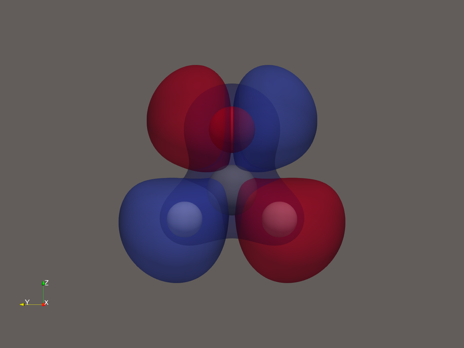
Open homo.cube, select its Gridded Data, and add a Contour with two isosurface values: 0.02 and -0.02. Tick Compute Scalars (click the gear icon to see it) and click Apply. Color the result by the orbital's values with the Cool to Warm preset, and set its Opacity to 0.6.
You should see: four lobes in the plane of the molecule, alternating red and blue for the orbital's two signs. One pair sits by the oxygen, on either side of the C=O bond. The other pair wraps the hydrogens, and at ±0.02 it is the larger of the two.
What you should see
Screenshot: Contour's properties with both values, and Compute Scalars under the gear icon
Screenshot to come: The Contour properties with the values 0.02 and -0.02, and Compute Scalars ticked, found under the gear icon
Step 5: Save a picture
Choose File ▸ Save Screenshot… and save to ~/scratch/orbitals-paraview.png at 1600 by 1200.
You should see: orbitals-paraview.png in the Files app, in your scratch folder. To make the same picture without clicking, run scripts/orbitals_paraview.py with pvbatch, from the folder holding the cube files.
Check your understanding
You raise the density isovalue from 0.0004 to 0.05. Does the surface get bigger or smaller, and why?
Smaller. The surface encloses only the places where the density is at least the isovalue. Density rises toward the nuclei, so a higher value is reached only close to the atoms and along the bonds.
Why does the orbital need two isosurfaces when the density needs only one?
An orbital's values are positive in some regions and negative in others, which is its phase. So one surface goes at +0.02 and another at −0.02. The density is never negative, so one surface is enough.
If something goes wrong
| What you see | Why | What to do |
|---|---|---|
| No surface at all | The isovalue is higher than any value in the file, or has the wrong sign | Try 0.05 for density, 0.02 and -0.02 for an orbital |
| Only one lobe of the orbital | Only one isosurface value was entered | Enter both 0.02 and -0.02 in Isosurfaces, then Apply |
| The atoms are specks | They're drawn at their size in ångströms on a ruler of grid steps | Set Atomic Radius Factor to 5.6, as in Step 3 |
| The orbital is one flat color | Compute Scalars is off, so there are no values to color by | Tick Compute Scalars under the gear icon, Apply, then color by the orbital's values |
Next
Credits
Cube files computed with PySCF (Apache-2.0) at B3LYP/6-31G(d), the level the Gaussian lessons use. Steps follow the ParaView 6.0.1 documentation. The isovalues here are the ones these lessons use, not a standard. Written for SBSC; text CC-BY 4.0.