
Status: draft. Verified steps and screenshots to come.
In this lesson you will draw streamlines that follow a velocity field, and add a second variable to the picture. Time: 10 minutes · Branch: Vector fields
Arrows give the direction of a flow at single points. Streamlines follow it, so recirculation, dead zones and mixing show up as shapes you can recognise. The same steps work on other vector fields: water velocity, magnetic fields, ion flux, wind.
Choose your program
Each version is a complete lesson on its own page. Pick the program you use.
| Program | Lesson | Practice data | The second variable | Minutes |
|---|---|---|---|---|
| ParaView | Draw streamlines in ParaView | disk_out_ref.ex2: air around a heated, spinning disk |
Temperature, colored along each line | 10 |
| MATLAB | Draw streamlines in MATLAB (page to come) | MATLAB's sample wind data |
Wind speed, colored along each line | 10 |
ParaView opens simulation output as written: Exodus, VTK, NetCDF, OpenFOAM and CSV. MATLAB suits velocity arrays that are already in MATLAB.
What each program's result looks like
Both pictures come from the lessons' own scripts.
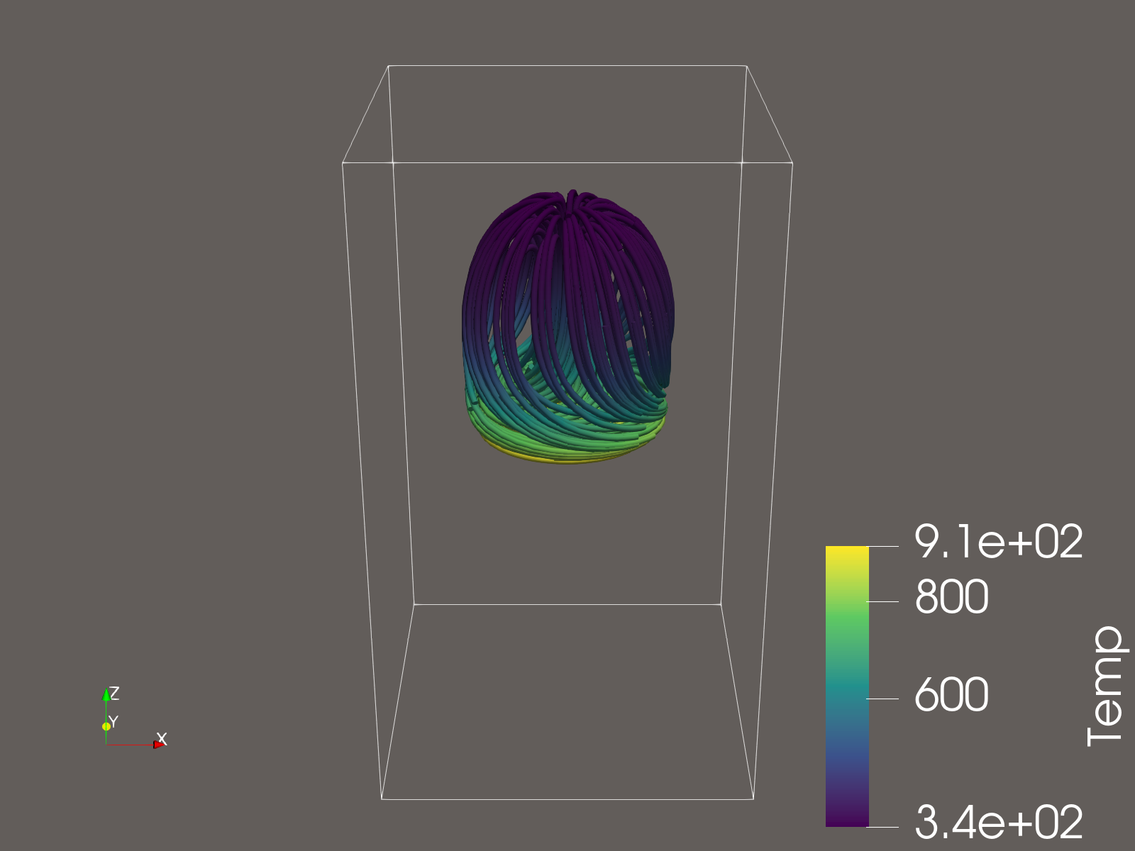
disk_out_ref.ex2, colored by temperature. Yellow is the hottest air.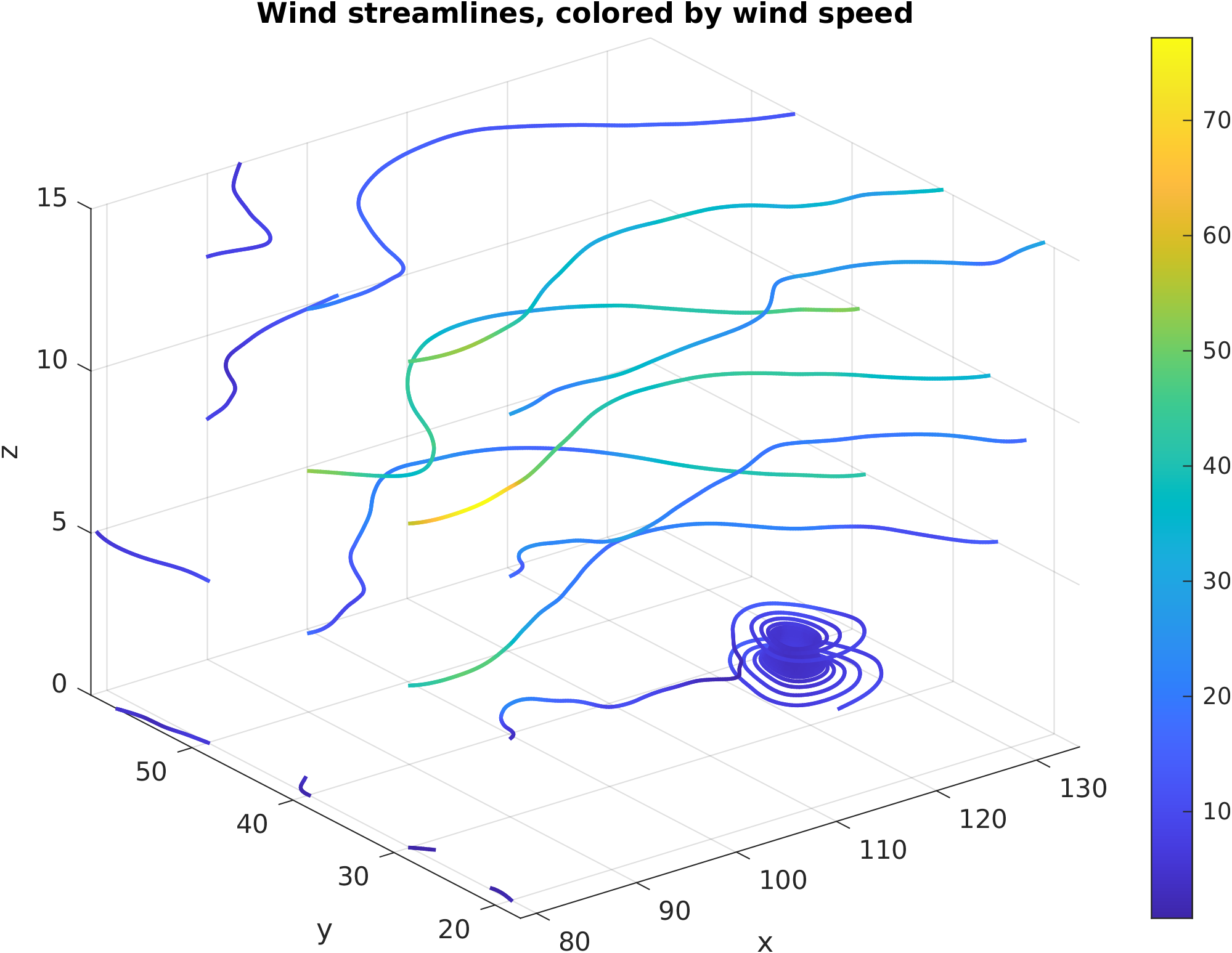
What every version teaches
Streamlines start from seeds. Each line is traced from a starting point, its seed, by following the flow direction step by step. The picture you get is therefore of the flow near the seeds, and nowhere else. If a region you care about looks empty, move or spread the seeds before deciding nothing happens there. Color the lines by a second variable, temperature or speed, and one picture carries both where the flow goes and what it carries.